JASP for Bayesian analyses with informative priors (using JAGS)
Ihnwhi Heo and Rens van de Schoot
Department of Methodology and Statistics, Utrecht University
Last modified: 30 September 2020
Welcome!
This tutorial illustrates how to perform Bayesian analyses in JASP (JASP Team, 2020) with informative priors using JAGS. Among many analytic options, we focus on the regression analysis and explain the effects of different prior specifications on regression coefficients. We also present the Shiny App designed to help users to define the prior distributions using the example in this tutorial. After the tutorial, we expect readers can understand how to incorporate prior knowledge in conducting Bayesian regression analysis to answer substantive research questions.
For readers who need fundamentals of JASP, we recommend following JASP for beginners. If readers are unfamiliar with the idea of Bayesian statistics and how to perform it with default JASP settings, we suggest reading JASP for Bayesian analyses with default priors. For readers who want to comprehend the Bayesian regression deeper, we advise you to follow Advanced Bayesian regression in JASP.
Since we continuously improve the tutorials, let us know if you discover mistakes, or if you have additional resources we can refer to. If you want to be the first to be informed about updates, follow Rens on Twitter.
Let’s get started!
How to cite this tutorial in APA style
Heo, I., & Van de Schoot, R. (2020, September). Tutorial: JASP for Bayesian analyses with informative priors (using JAGS). Zenodo. https://doi.org/10.5281/zenodo.4032757
PhD-Delays Dataset
We will use a phd-delay dataset (Van de Schoot, 2020) from Van de Schoot, Yerkes, Mouw, and Sonneveld (2013). To download the dataset, click here.
The dataset is based on a study that asks Ph.D. recipients how long it took them to complete their Ph.D. projects (n = 333). It turned out that the Ph.D. recipients took an average of 59.8 months to finish their Ph.D. trajectory.
For more information on the sample, instruments, methodology, and research context, we refer interested readers to the paper (see references). A brief description of the variables in the dataset follows. The variable names in the table below will be used in the tutorial, henceforth.
| Variable name | Description |
|---|---|
| B3_difference_extra | The difference between planned and actual project time in months |
| E4_having_child | Whether there are any children under the age of 18 living in the household (0 = no, 1 = yes) |
| E21_sex | Respondents’ gender (0 = female, 1 = male) |
| E22_Age | Respondents’ age |
| E22_Age_Squared | Respondents’ age-squared |
How to cite the dataset in APA style
Van de Schoot, R. (2020). PhD-delay Dataset for Online Stats Training [Data set]. Zenodo. https://doi.org/10.5281/zenodo.3999424
I. Setting a goal: A research question
- Earning a Ph.D. degree is a long and enduring process. Many factors are involved in timely completion, abrupt termination, or some delay of the Ph.D. life. For the current tutorial, we examine how age is related to the Ph.D. delay.
- Let’s think about the relationship between age and Ph.D. delay. Do you think they are linearly related? Are there any different ideas such that the age is non-linearly associated with the delay? We expect the relationship between the completion time and age are non-linear. This might be because, at a certain point in your life (say mid-thirties), family life takes up more of your time compared to when you are in the twenties.
- To that end, we examine whether the age of the Ph.D. recipients predicts a delay in their Ph.D. projects. The regression model is consequently the one we should adopt to answer the research question. We use the difference variable (B3_difference_extra) as the dependent variable and the age (E22_Age) and the age-squared (E22_Age_Squared) as the independent variables for the regression model.
II. Eyes on the dataset
1. Loading data
- The statistical analysis goes hand in hand with data. If you have not yet downloaded the dataset for our tutorial, click here.
- JASP offers three ways to load the data with simple mouse clicks: from your computer, the in-built data library, or the Open Science Framework.
- If you are not familiar with loading the data, please go to JASP for beginners and see how to load the data.
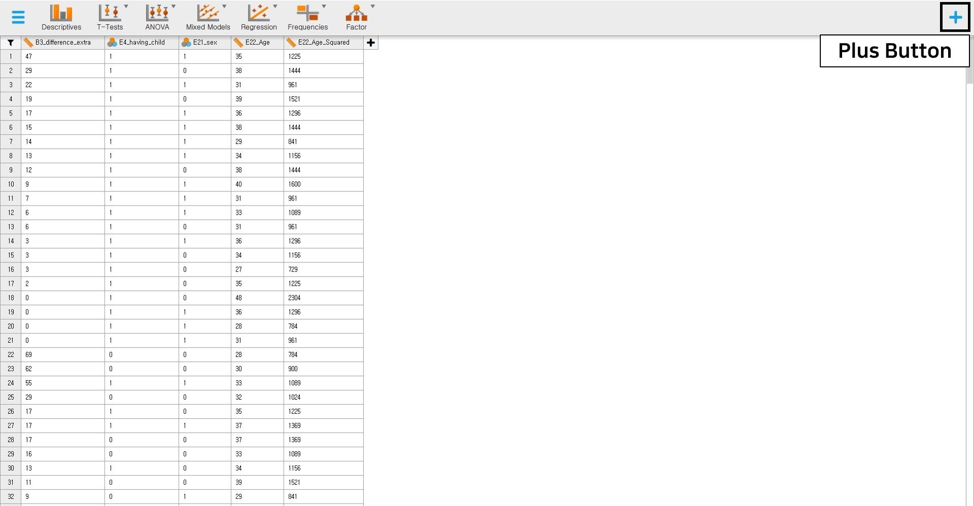
- It’s time to meet the data in JASP. Did you successfully load your dataset? The column names should correspond to the names of the five variables in the dataset.

2. Exploring and inspecting data
- It is always desirable to explore your data once loaded. We can inspect via either descriptive statistics or data visualization.
- If you are not familiar with data exploration, please go to JASP for beginners and check how to inspect the data.
Descriptive statistics
- Let’s see the descriptive statistics of the variables to check whether all the data points make sense.
- Click Descriptives at the top bar to proceed with -> Move all the variables to space under the Variables section -> Check Frequency tables (nominal and ordinal variables) -> Click Statistics -> Check additional descriptive statistics (S. E. mean under Dispersion, Median under Central Tendency, and Skewness and Kurtosis under Distribution) for better understanding.

- For all the variables, the sample size is 333 without any missing values.
- For the difference variable (B3_difference_extra), the mean and the standard error of the mean are 9.97 and 0.79.
- For the age variable (E22_Age), the mean and the standard error of the mean are 31.68 and 0.38.
- For the age-squared variable (E22_Age_Squared), the mean and the standard error of the mean are 1050.22 and 35.97.
- For the dichotomous variables (E4_having_child and E21_sex), frequency tables are presented.
- Given the descriptive statistics, all the data points substantively make sense.
Data visualization
- Let’s plot the expected relationship between age and the delay for visual inspection. To do that, we need to remain only two variables, B3_difference_extra and E22_Age, under the Variables section.

- Click Plots and check Scatter Plots -> Under Scatter Plots, uncheck Show confidence interval 95.0%. We can see the scatter plot between the difference variable on the x-axis and the age variable on the y-axis.
- Although we can use this scatter plot for our visual inspection purposes, it might be better to locate the difference variable on the y-axis and the age variable on the x-axis since we regress the difference variable on the age variable. We can simply do that by changing the variable order under the Variables section: set E22_Age to be the first and B3_difference_extra the latter.

- With this plot, we can see the non-linear relationship between the difference variable and the age variable.
- It is also possible to examine the linear relationship by drawing the linear regression line. How? Uncheck Smooth and check Linear under Add regression line. Can you see the linear line?

III. Intermezzo: Parameter estimation and hypothesis testing from a Bayesian perspective
1. Bayesian parameter estimation
- A notable feature of Bayesian statistics is that the prior distributions of parameters are combined with the likelihood of data to update the prior distributions to the posterior distributions (see Van de Schoot et al., 2014 for introduction and application of Bayesian analysis). The updated posterior distributions are materials for Bayesian statistical inference. This logic implies the crucial role of prior distributions in doing Bayesian statistics!
- In our regression model, parameters are the intercept, two regression coefficients, and residual variance. Thus, we should specify the prior distributions for the intercept, two regression coefficients, and residual variance, respectively.
- Please note that we leave the discussion about priors for the intercept and the residual variance untouched in this exercise. We thus consider the prior distributions for the regression coefficients only.
- Let’s think about the model under consideration to see what the regression coefficients are. The regression formula for the current example can be written as: \(Difference = b_{0} + beta_{Age} * X_{Age} + beta_{Age-squared} * X_{Age-squared}\)
- You can see that the regression coefficients are \(beta_{Age}\) and \(beta_{Age-squared}\) whereas \(b_{0}\) is the intercept.
- The regression coefficients you will see in the output panel are the summaries of the posterior distributions of these two regression coefficients.
2. Bayesian hypothesis testing
- Bayesian hypothesis testing focuses on which hypothesis receives relatively more support from the observed data. This is quantified by the Bayes factor (Kass & Raftery, 1995).
- If the Bayes factor in favor of the alternative hypothesis is 15, this means that the support in the observed data is about fifteen times larger for the alternative hypothesis than for the null hypothesis. As you can see, how likely the data are to be observed among competing hypotheses is expressed in terms of the Bayes factor.
- Please note that we do not use such words as significant and p-value in Bayesian hypothesis testing. They are the words used under the frequentist framework.
3. Setting seed values for reproducible results
- Bayesian inference is based on the posterior distribution of parameters after taking into account the likelihood of data and the prior distribution. The likelihood and the prior are expressed in terms of mathematical functions.
- The potential problem that could arise is that, usually, the posterior distribution is hard to get analytically (see Chapter 5 and Chapter 6 in Kruschke, 2014 for information about conjugate and non-conjugate prior). To solve this issue, Bayesian statistics uses the random number generator to approximate the posterior distribution. Due to generating random numbers, results from Bayesian analyses are slightly different each time we run Bayesian analyses.
- Surprisingly, this is not completely random such that each software has its hidden rule that the sequence of numbers is generated! We can thus say the software is based on a pseudorandom number generator. The idea is that, whenever a certain number is fed as an input to the generator, the software produces the same sequence of pseudorandom numbers. Therefore, researchers and statisticians feed a specific number to the statistical software to make it reproduce the same outputs. This is why we set seed to get reproducible results.
- For more information about the setting seed values for Bayesian statistics, see Chapter 7 in Kruschke (2014).
IV. Regression with default priors
- Let’s first proceed with the analyses with the default priors. Why? The reason is to compare the prior specifications between default and informative priors, later.
- Default prior settings can be taken into account, for instance, when researchers have no knowledge or cannot find relevant previous studies about the parameters of interest. This choice, however, should be taken with concerns (see Van De Schoot, Broere, Perryck, Zondervan-Zwijnenburg, & Van Loey, 2015 for caution in using default priors).
- JAGS does not provide the default prior settings. We, thus, have to think about the type of prior distributions and their hyperparameters for our regression model. Hyperparameters are the parameters for the prior distributions.
1. Choosing default prior distributions and their hyperparameters
Regression coefficients
- We follow the default prior specifications that the R package blavaan uses with the JAGS target (Merkle, & Rosseel, 2018). You can find more information in the tutorial Bayesian regression in blavaan (using JAGS).
- In blavaan, the normal prior \(\mathcal{N}(\mu, \ 1/\sigma^{2})\), where \(\mu\) is the mean and \(\ 1/\sigma^{2}\) is the precision of the distribution, is used for the regression coefficient.
- “Wait, what is the precision? Should it be the variance?” A great question! JAGS uses the precision instead of the variance. The precision is the inverse of the variance. For example, the precision of 0.01 is equal to the variance of 100 (the inverse of 0.01 is 100).
- Blavaan uses 0 and 1e-2 (1e-2 is equal to \(1 × 10^{-2}\), which is 0.01) as the mean and the precision for the prior distribution for regression coefficients. Since the mean 0 and the precision 1e-2 are the parameters for the prior distribution, they are hyperparameters. In summary, we set \(\mathcal{N}(0, 1/100)\) as our prior distributions for both regression coefficients.
Intercept
- Although we leave intercept and residual variance untouched, we have to specify the prior distributions for the intercept and the residual variance to run JAGS (otherwise, JAGS does not work!).
- We again refer to the default priors that blavaan uses for the intercept: the normal prior distribution \(\mathcal{N}(\mu_0, \ 1/\sigma^{2}_{0})\), where \(\mu_0\) is the mean and \(\ 1/\sigma^{2}_{0}\) is the precision of the distribution.
- Blavaan uses 0 and 1e-3 (1e-3 is equal to \(1 × 10^{-3}\), which is 0.001) as hyperparameters for the mean and the precision, respectively. That is, we set \(\mathcal{N}(0, 1/1000)\) as our prior distribution for the intercept.
Residual variance
- In a normal regression model, the inverse gamma distribution is used as a prior for the variance thanks to the conjugacy (Lynch, 2007). Keep in mind, however, that JAGS uses precision instead of the variance. Therefore, we have to consider prior distributions for the precision.
- To do that, we should use the gamma distribution as a prior for the precision. In other words, using a gamma distribution on the precision is the same as using an inverse gamma distribution on the variance (think about the inverse relationship!). Note that blavaan also places prior distributions on the precision instead of the variance for the residual variance.
- The gamma distribution looks like \(Gamma(\kappa_0,\theta_0)\), where \(\kappa_0\) is the shape parameter and \(\theta_0\) the rate parameter of the distribution.
- As hyperparameters, let’s use 0.5 for both shape and rate parameter. This setting is an uninformative prior for the precision, which has been found to perform well. In other words, we set \(Gamma(.5, .5)\) as our prior distribution for the precision.
2. Running JAGS
- To run the model, we have to type the JAGS code that species the model in JASP.
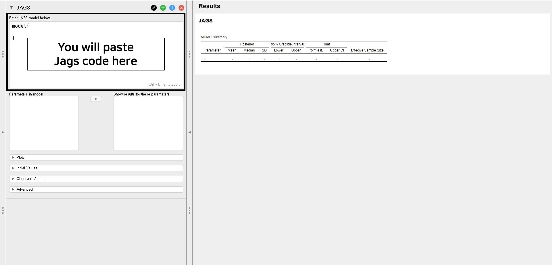
- If you click the JAGS button on the top bar, you encounter the control panel to feed the code under Enter JAGS model below.
JAGS grammar: A primer
- In writing the JAGS code, we have to follow the JAGS grammar. Although we list a couple of them, readers can find the extensive JAGS manual at the mcmc-jags project. We also refer readers to RJAGS: how to get started that illustrates how to run the JAGS but in R.
- The two main pillars that consist of JAGS model specification are the likelihood and the prior.
- For the likelihood, we specify the model of interest: the regression model in our case.
- For the prior, we specify the type of distribution (e.g., normal distribution, gamma distribution) with its hyperparameters.
- To that end, the JAGS model that we use can be specified as:
model{
    # likelihood
    for (i in 1:333){
    mu[i] <- intercept + beta1 * E22_Age[i] + beta2 * E22_Age_Squared[i]
    B3_difference_extra[i] ~ dnorm(mu[i],tau)
    }

    # priors
    intercept ~ dnorm(0,1e-3)
    beta1 ~ dnorm(0,1e-2)
    beta2 ~ dnorm(0,1e-2)
    tau ~ dgamma(0.5,0.5)
}- Did you notice that there are two pillars in the JAGS model specification, which are the likelihood and the prior? They are guided with the number sign (#).
- In the code, intercept, beta1, beta2, and tau are the parameters.
- The regression coefficients for the age and the age-squared variable are beta1 and beta2, respectively.
- Tau is the precision parameter, which is the inverse of the variance.
- In the likelihood, 333 in ‘for (i in 1:333)’ is equal to the sample size. The alphabet i corresponds to each row in the dataset.
- The tilde (~) sign means ‘follow’.
- beta1 ~ dnorm(0,1e-2) means that the regression coefficient of the age variable follows the normal distribution with the mean of 0 and the precision of 0.01.
- Such terms as dnorm and dgamma refer to the density of the normal distribution and the density of the gamma distribution.
- Copy and paste the code into the Enter JAGS model below section.
Set a seed value and the number of iterations
- Before running this code, we set the seed and the number of iterations.
- Regarding a seed, let’s use a seed value of 123 for replicable results. To do that, click the Advanced option in the control panel. Below Repeatability, type 123 for the seed.
- The initial number of burnin samples and that of samples to take are 500 and 2000, respectively. For our example, we use 5000 burnin samples and take additional 20000 samples. Under MCMC parameters of the Advanced option, type 20000 in No. samples (i.e., the number of samples) and 5000 in No. burnin samples (i.e., the number of burin samples). In total, we do 25000 iterations.
- We keep using the seed value of 123 and the number of iterations for subsequent analyses.
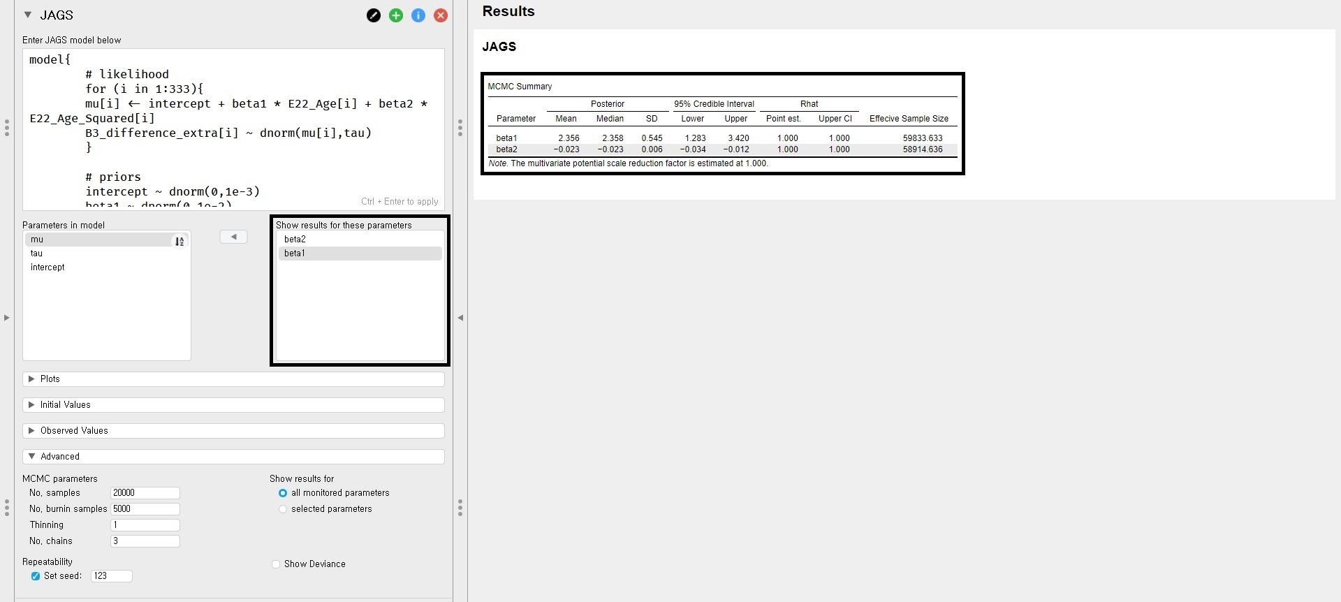
- If you have followed what is illustrated, your JASP screen should look like the snapshot below.
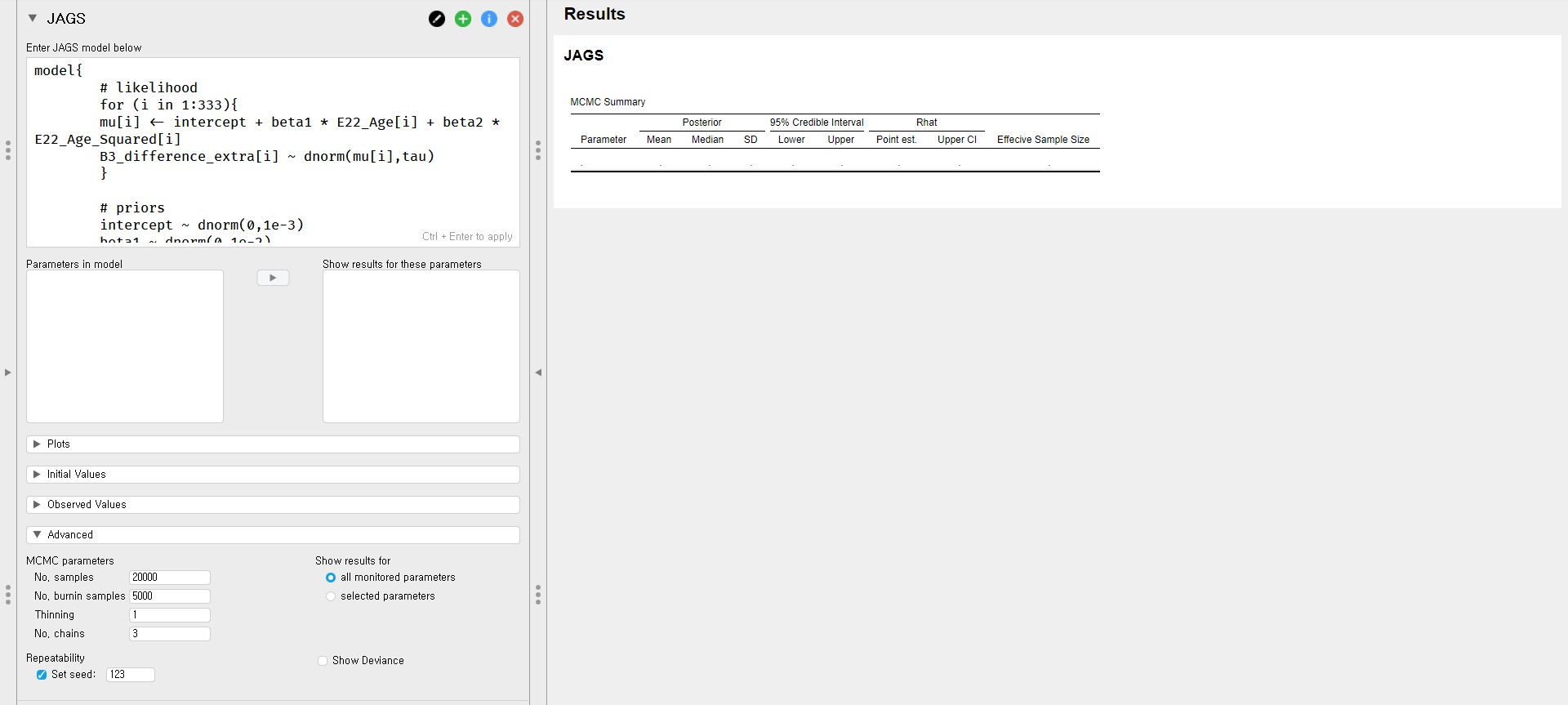
- Hope we are looking at the same screen! Go again to the code that we have pasted (i.e., the Enter JAGS model below section). Press Ctrl and Enter on the keyboard together to apply the code. With this action, you are running the model that we specified!
- Shortly, we can see a list of parameters under the Parameters in model in the control panel. This means that the posterior distributions for regression parameters are obtained by JAGS.
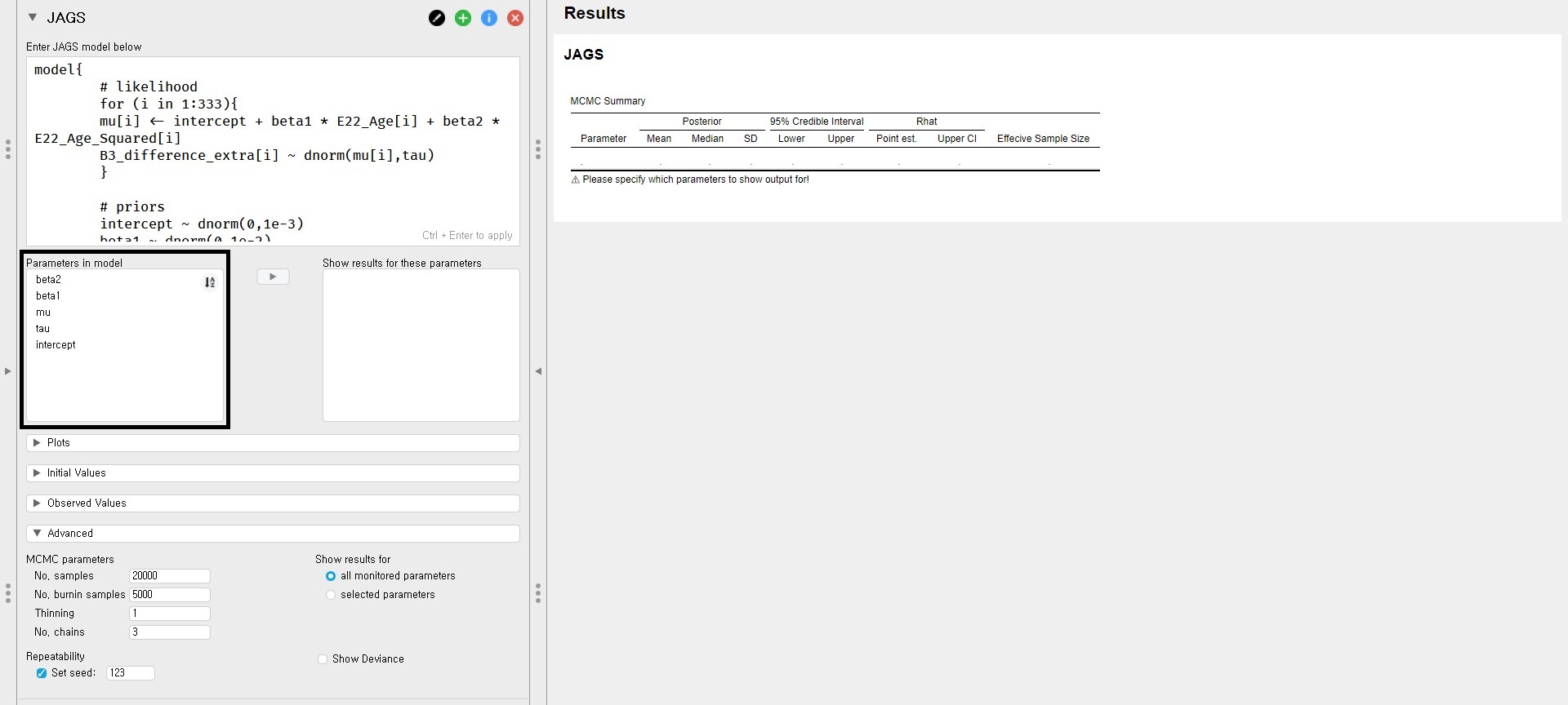
- As we are interested in the posterior distributions of two regression coefficients (i.e., the age and the age-squared variable), move beta1 and beta2 into the Show results for these parameters section on the right. After a few seconds, JASP presents the MCMC Summary table on the output panel.
Interpretation of the output
- We can find a summary of regression coefficients in the MCMC Summary table. The table presents the posterior distribution of regression coefficients after considering the default priors for age and age-squared variable and the likelihood of the data.
- The posterior mean of the regression coefficient of age (beta1) is 2.356. We can interpret this value such that a one-year increase in age adds about 2.356 delays in Ph.D. projects on average. The 95% credible interval of age is [1.283, 3.420], which means that there is a 95% probability that the regression coefficient of age lies in the population with the corresponding credible interval. We also notice that a 95% credible interval does not include 0, which shows the evidence of the effect of age in predicting the Ph.D. delay.
- The posterior mean of the regression coefficient of age-squared (beta2) is -0.023. This can be interpreted such that one unit increase of the age-squared variable leads to a decrease of 0.023 unit in the Ph.D. delay on average. The 95% credible interval of [-0.034, -0.012] indicates that we are 95% sure that the regression coefficient of age-squared lies within the corresponding interval in the population. Did you notice that 0 is not included in the interval? Therefore, it is fairly sure that there is an effect of the age-squared variable in predicting the delay.
- If you are curious about examining convergence diagnostics, please go to WAMBS Checklist in JASP (using JAGS).
V. Regression with informative priors
- Now, it’s time to specify the informative priors. One might think that the informative priors are always preferred over the default priors since it is ‘informative’, hence decorating the outputs in a more meaningful way. However, this approach is dangerous. We should use informative priors when there are reliable sources for the prior information (e.g., previous literature and expert knowledge). Otherwise, the conclusion becomes arbitrary. It is also important to note that specifying the informative priors should be done before peeking at the data. You are double-dipping, otherwise. Therefore, researchers have to be aware of what they are doing when working with the informative priors!
1. Adjusting hyperparameters for regression coefficients
- From now on, we try four different prior specifications for the regression coefficients of age and age-squared variable. Let’s keep using the normal distribution as the type of distribution, so we only adjust the hyperparameters for the mean and the precision.
- In specifying the precision, we use the form of ‘1/variance’ since variance is more intuitive than precision for us.
- The mean of the prior distribution indicates a parameter value that we deem most likely. The precision expresses how certain we are about the mean. For example, lower precision (thus, higher variance) means we are uncertain about the mean. If we choose to use higher precision (hence, lower variance), this indicates we are certain about the mean.
- In implementing the follow-up prior specifications, copy and paste the following code into the Enter JAGS model below section. Next, never forget to press Ctrl and Enter together to apply the code. Otherwise, the changes might not be applied!
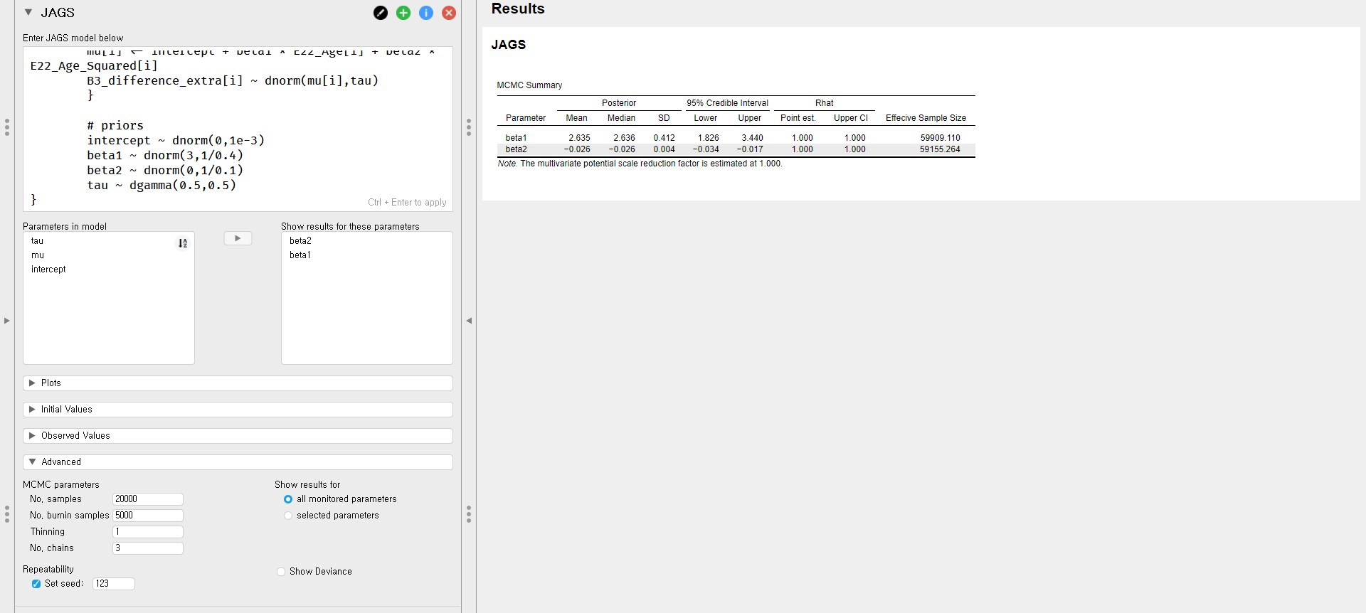
beta1 ~ N(3, 1/0.4) and beta2 ~ N(0, 1/0.1)
model{
    # likelihood
    for (i in 1:333){
    mu[i] <- intercept + beta1 * E22_Age[i] + beta2 * E22_Age_Squared[i]
    B3_difference_extra[i] ~ dnorm(mu[i],tau)
    }

    # priors
    intercept ~ dnorm(0,1e-3)
    beta1 ~ dnorm(3,1/0.4)
    beta2 ~ dnorm(0,1/0.1)
    tau ~ dgamma(0.5,0.5)
}
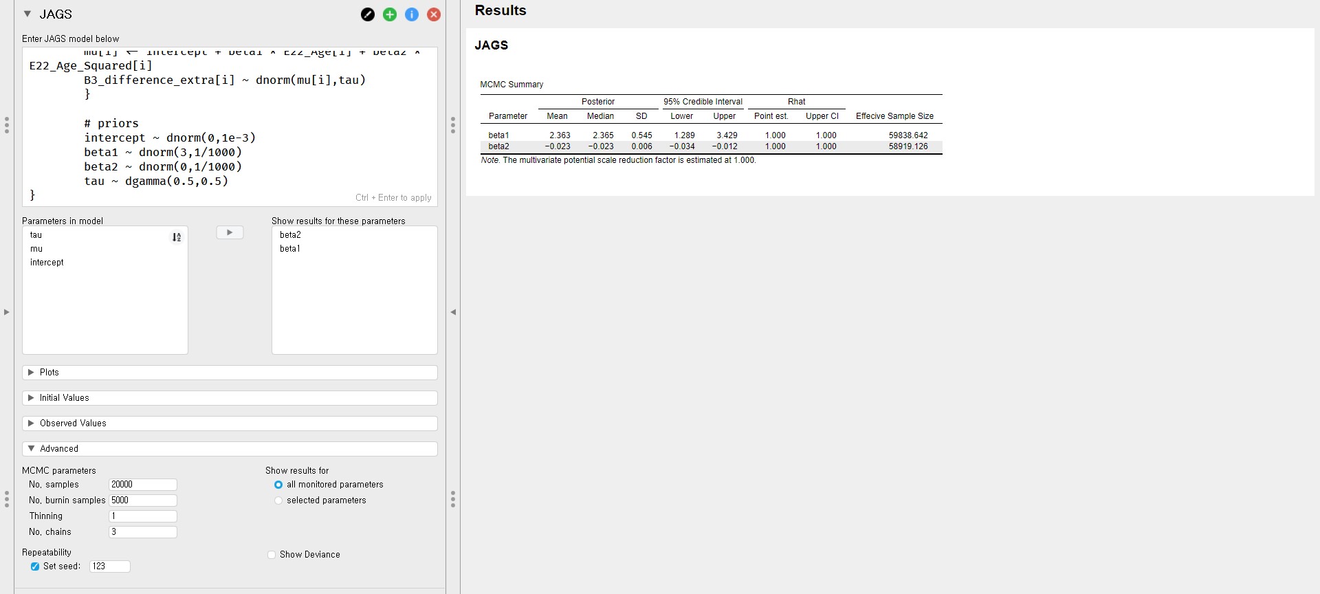
beta1 ~ N(3, 1/1000) and beta2 ~ N(0, 1/1000)
model{
    # likelihood
    for (i in 1:333){
    mu[i] <- intercept + beta1 * E22_Age[i] + beta2 * E22_Age_Squared[i]
    B3_difference_extra[i] ~ dnorm(mu[i],tau)
    }

    # priors
    intercept ~ dnorm(0,1e-3)
    beta1 ~ dnorm(3,1/1000)
    beta2 ~ dnorm(0,1/1000)
    tau ~ dgamma(0.5,0.5)
}
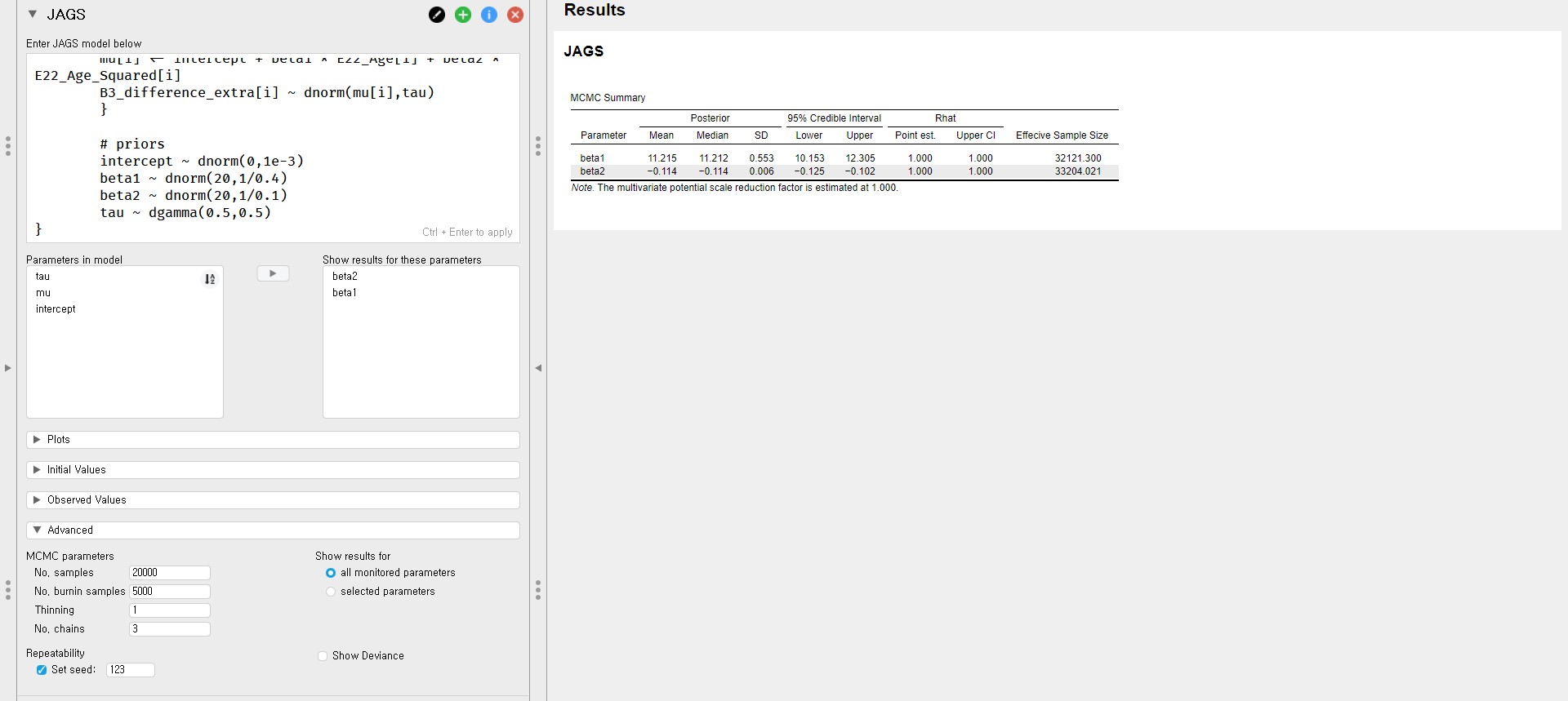
beta1 ~ N(20, 1/0.4) and beta2 ~ N(20, 1/0.1)
model{
    # likelihood
    for (i in 1:333){
    mu[i] <- intercept + beta1 * E22_Age[i] + beta2 * E22_Age_Squared[i]
    B3_difference_extra[i] ~ dnorm(mu[i],tau)
    }

    # priors
    intercept ~ dnorm(0,1e-3)
    beta1 ~ dnorm(20,1/0.4)
    beta2 ~ dnorm(20,1/0.1)
    tau ~ dgamma(0.5,0.5)
}
beta1 ~ N(20, 1/1000) and beta2 ~ N(20, 1/1000)
model{
    # likelihood
    for (i in 1:333){
    mu[i] <- intercept + beta1 * E22_Age[i] + beta2 * E22_Age_Squared[i]
    B3_difference_extra[i] ~ dnorm(mu[i],tau)
    }

    # priors
    intercept ~ dnorm(0,1e-3)
    beta1 ~ dnorm(20,1/1000)
    beta2 ~ dnorm(20,1/1000)
    tau ~ dgamma(0.5,0.5)
}
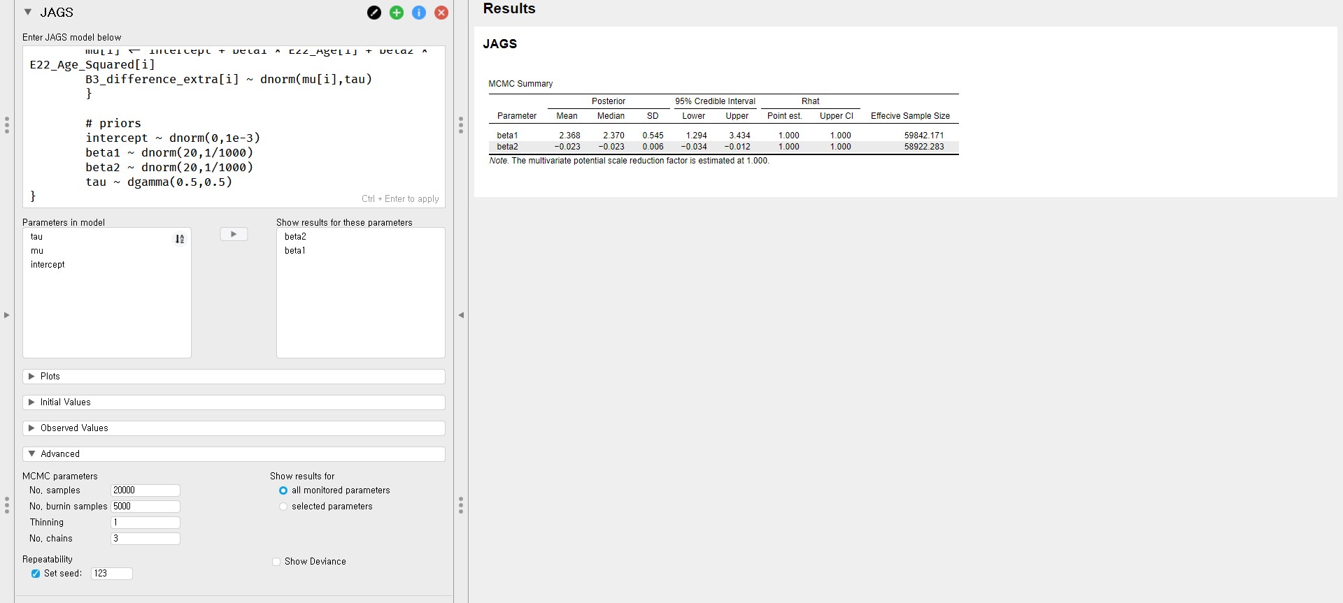
Summary of the posterior mean and the posterior standard deviation
| \(Age\) | Default: \(\mathcal{N}(0, 1e-2)\) | \(\mathcal{N}(3, 1/0.4)\) | \(\mathcal{N}(3, 1/1000)\) | \(\mathcal{N}(20, 1/0.4)\) | \(\mathcal{N}(20, 1/1000)\) |
|---|---|---|---|---|---|
| Posterior mean | 2.356 | 2.635 | 2.363 | 11.215 | 2.368 |
| Posterior standard deviation | 0.545 | 0.412 | 0.545 | 0.553 | 0.545 |
| \(Age^2\) | Default: \(\mathcal{N}(0, 1e-2)\) | \(\mathcal{N}(0, 1/0.1)\) | \(\mathcal{N}(0, 1/1000)\) | \(\mathcal{N}(20, 1/0.1)\) | \(\mathcal{N}(20, 1/1000)\) |
|---|---|---|---|---|---|
| Posterior mean | -0.023 | -0.026 | -0.023 | -0.114 | -0.023 |
| Posterior standard deviation | 0.006 | 0.004 | 0.006 | 0.006 | 0.006 |
2. Effect of informative prior specifications on parameter estimation
- Can we compare the results of parameter estimation stemmed from different prior specifications? Of course, we can! We check two things: the relative bias and the change of parameter estimates.
Relative bias
- Relative bias can be used to express the difference between the default prior and the informative prior.
- The formula for the relative bias follows: \(bias = 100*\frac{(model \; with \; specified \; priors\; – \; model \; with \; default \;priors)}{model \; with \; default \; priors}\)
- To preserve clarity, we will just calculate the bias of the two regression coefficients and only compare the model with the default prior and the model that uses \(\mathcal{N}(20, 1/0.4)\) for the age variable and \(\mathcal{N}(20, 1/0.1)\) for the age-squared variable as informative priors.
- For the age variable, the relative bias is \(100*\frac{(11.215\; – \; 2.356)}{2.356}\). This equals 376.02%.
- For the age-squared variable, the relative bias is \(100*\frac{(-0.114\; – \; (-0.023))}{-0.023}\), which equals 395.65%.
- The influence of the informative prior is around 376.02% for the age variable and 395.65% for the age-squared variable. This signals a tremendous change in the results with different prior specifications. For the concrete examination, let’s take a look at the parameter estimates.
Parameter estimates
- See the posterior mean, the posterior standard deviation, and the 95% credible interval from the MCMC Summary table.
| \(Age\) | Default: \(\mathcal{N}(0, 1e-2)\) | Informative: \(\mathcal{N}(20, 1/0.4)\) |
|---|---|---|
| Posterior mean | 2.356 | 11.215 |
| Posterior standard deviation | 0.545 | 0.553 |
| 95% credible interval | [1.283, 3.420] | [10.153, 12.305] |
| \(Age^2\) | Default: \(\mathcal{N}(0, 1e-2)\) | Informative: \(\mathcal{N}(20, 1/0.1)\) |
|---|---|---|
| Posterior mean | -0.023 | -0.114 |
| Posterior standard deviation | 0.006 | 0.006 |
| 95% credible interval | [-0.034, -0.012] | [-0.125, -0.102] |
- For both variables, there are changes in the parameter estimates. For instance, a one-year increase in age adds about 2.356 delays in Ph.D. projects on average under the default prior. When the informative prior is used, a one-year increase in age adds about 11.215 delays on average!
3. Conclusion about the effect of different prior specifications
- Given the relative bias and the parameter estimates, we conclude that there exist differences due to different prior specifications. Therefore, using different prior distributions would not end up with similar conclusions.
- The influence of prior also depends on the size of the dataset. The sample size is 333 for our data, which is relatively big. When the dataset is big, the influence of the prior becomes relatively small. If one would have a smaller dataset, on the other hand, the influence of the prior becomes relatively larger.
4. Do it yourself with the Shiny App!
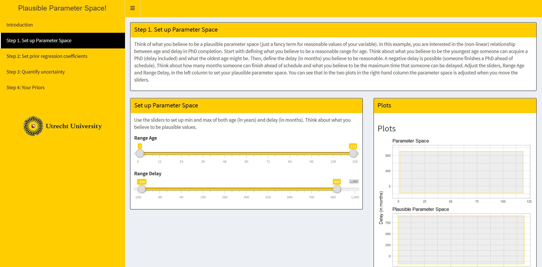
- It is the best learning to practice and experience the actual process by oneself. We introduce a very useful Shiny App (Smeets & Van de Schoot, 2020)! It enables readers to adjust prior distributions for the regression coefficients for the age and the age-squared variable using the Ph.D. delay dataset.
- The Shiny App is self-explanatory and provides interactive plots. We hope readers can get an intuition about what they are doing in specifying prior distributions.
- Click here to launch the Shiny App!
VI. Epilogue
- Congratulations! We are standing at the endpoint. We hope you found this tutorial useful.
- If you are curious about a deeper side of Bayesian regression, we recommend following the tutorial Advanced Bayesian regression in JASP. It provides readers with an in-depth illustration of outputs and other options in conducting Bayesian regression analysis.
- For readers who plan to implement Bayesian analyses for their own data, we suggest following the procedures explained in the tutorial WAMBS Checklist in JASP (using JAGS). It guides you to sensibly apply Bayesian statistics in answering substantive research questions thoroughly.
References
JASP Team (2020). JASP (Version 0.13.1)[Computer software].
Kruschke, J. (2014). Doing Bayesian data analysis: A tutorial with R, JAGS, and Stan (2nd ed.). Academic Press.
Lynch, S. M. (2007). Introduction to applied Bayesian statistics and estimation for social scientists. Springer Science & Business Media.
Merkle, E., & Rosseel, Y. (2018). blavaan: Bayesian Structural Equation Models via Parameter Expansion. Journal of Statistical Software, 85(4), 1–30. https://doi.org/10.18637/jss.v085.i04
Smeets, L., & Van de Schoot, R. (2020, September 15). Code for the ShinyApp to Determine the Plausible Parameter Space for the PhD-delay Data (Version v1.0). Zenodo. https://doi.org/10.5281/zenodo.4030288
Van de Schoot, R. (2020). PhD-delay Dataset for Online Stats Training [Data set]. Zenodo. https://doi.org/10.5281/zenodo.3999424
Van de Schoot, R., Broere, J. J., Perryck, K. H., Zondervan-Zwijnenburg, M., & Van Loey, N. E. (2015). Analyzing small data sets using Bayesian estimation: The case of posttraumatic stress symptoms following mechanical ventilation in burn survivors. European Journal of Psychotraumatology, 6(1), 25216. https://doi.org/10.3402/ejpt.v6.25216
Van de Schoot, R., Kaplan, D., Denissen, J., Asendorpf, J. B., Neyer, F. J., & Van Aken, M. A. (2014). A gentle introduction to Bayesian analysis: Applications to developmental research. Child development, 85(3), 842-860. https://doi.org/10.1111/cdev.12169
Van de Schoot, R., Yerkes, M. A., Mouw, J. M., & Sonneveld, H. (2013). What took them so long? Explaining PhD delays among doctoral candidates. PloS one, 8(7), e68839. https://doi.org/10.1371/journal.pone.0068839


